Table of Contents
Convolutional Neural Networks
“In deep learning, a convolutional neural network is a class of deep neural networks, most commonly applied to analyzing visual imagery. “ (Valueva)
A convolutional neural network, also known as CNN, is a type of neural network the specializes in processing grid-like topology, such as an image. In this workshop we will be going over neural networks and their structure. We will also take a look at their individual components and examine why they are so good for image classification problems.
CNN vs NN
If we look back to our previous workshop, we classified different clothing items using a simple neural network. While our objective was easy, what happens when we want to classifiy more complex images? How do we create a neural network that given images of a couple models of cars, can classify any type of car?
Neural networks are limited in image classification applications because they aren’t tailored for image classification applications. We aren’t extracting any valuable information when implementing neural networks, we’re more so going through the trial and error of trying to define what an image is. While this method is effective for simple images, when we introduce harder classification problems, neural networks will fail
A CNN on the other hand, implements a different method; feature extraction. A CNN will look through images and extract features that classify an object in an image as is. Instead of trying to memorize what an object resembles, it will gather key feature information of an object.
What do you mean by feature extraction?
Take a look at the following image and take a second to observe what you see.

A good chunk of you might mention that you see a man looking forward. Another subset might mention they see a man looking right. In this case both answers are right because it’s an optical illusion. This optical illusion is meant to distort the viewers perception based on where they draw their eyes towards.
If you look at his nose, you will see an man looking to the right. If you look at his ears, you will see a man looking straight ahead.
Our head makes this distinction because we classify the things we see based on different features. Depending on what feature you see, your brain will percieve the image differently.
CNNs do the same. They look to extract different features from an image in order to understand what type of image they are looking at. This feature extraction allows for a more robust image classification model.
What is the structure of a CNN?
While I won’t be going in depth into the math behind a CNN, you can check this paper out as it clearly explains the theory behind a CNN for beginners.
Let’s take a look at the basic structure of a CNN.
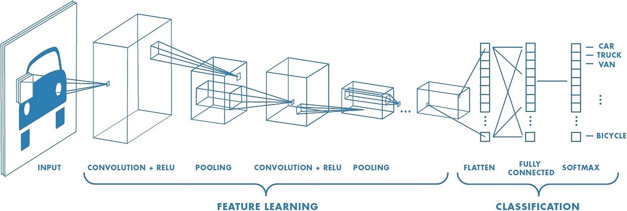
The structure above is of a simple CNN. There are different variations to how a CNN is implemented, the one pictured above is a simple implementation.
The process of a CNN starts with a feature learning process that learns different features of images, and the second classification portion is a standard fully connected neural network.
Convolution
The first step of a CNN is to take an image and derive a feature map using a kernel.
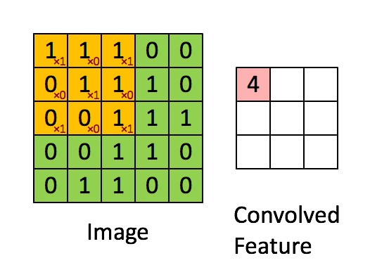
Above we can see the process occuring. On the left we have an image - each box represents a pixel value. We can also see a yellow box iterating through the image - this is our kernel. The kernel takes a subset of the image and extracts a point of the feature map. These results get carried over and placed into the feature map respectively.
Since our kernel only moves 1 block at a time we say our kernel has a stride of 1.
Let’s take a look at how the example above derives the values. Here we have our kernel:
K = [[1 , 0 , 1],
      0 , 1 , 0],
      1 , 0 , 1]]
Our image is defined as:
Img = [[1, 1, 1, 0, 0],
        0, 1, 1, 1, 0],
        0, 0, 1, 1, 1],
        0, 0, 1, 1, 0],
        0, 1, 1, 0, 0]]
In order to get every value in the feature map, for every time the kernel moves, we multiply each point together and sum it up. This gives us the following value for the first feature map point:
1*1 + 1*0 + 1*1
0*0 + 1*1 + 0*1
1*0 + 1*0 + 1*1
That value is equal to 4 so our feature map point on the top left is 4
So now we have a feature map - so what?
Well the first thing to take into account is that now our image is smaller. Remember when we’re working with a 28x28 image, when flattened that turned into 784 nodes in our input layer. By doing this we are able to scale the image down and extract only import features. Typically in our feature map(convolved feature), the higher the value the more significant a feature was and if we remember from the first example, our brain is able to identify things mostly based on features. This feature map helps us to preserve the important features.
How are the Kernel values determined Well initially the kernel values seem to be initialized randomly. Like weights in a neural network, the kernel updates itself and learns to pick up different features.
Is there only one feature map? The most important thing to note here is that there are going to be a different amount of feature maps created. Each feature map will have extracted its own feature.
Now let’s see what this process would look like on a 3d image(color image)
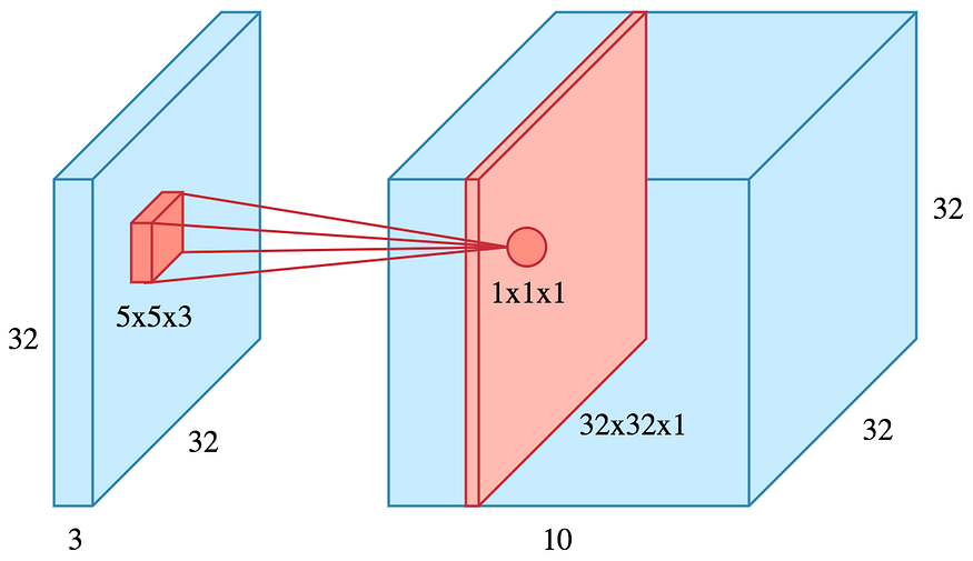
Here we are applying the same process as mentioned except this it what it really looks like. In this example a 5x5x3 kernel is used to convolve the image and creates 32 different feature maps. Ideally each feature map would pick up a different feature from the training set. Since the kernel is 3 dimensions, each dimension’s kernel result is added, and the sum of those 3 values creates 1 value. So there, we go from 3 dimensions to 1 dimension.
ReLU Layer
For a model to really be powerful, non-linearity needs to be introduced. Since images are naturally non-linear, we want to apply an activation function to make our feature maps non-linear.
Simply, we want our image to not have a gradual change in colors, but rather for everything to be more abrupt(non-linear).
When we run mathematical operations on our image, we risk introducing linearity so to counter that, we apply an activation function such as relu. Since ReLU itself is nonlinear(not a straight line), by applying it we can make our feature map non-linear.
Pooling Layer
there are different types of pooling methods, but for this workshop we will only be going over max pooling.
“After a convolution operation we usually perform pooling to reduce the dimensionality. This enables us to reduce the number of parameters, which both shortens the training time and combats overfitting. Pooling layers downsample each feature map independently, reducing the height and width, keeping the depth intact.”
Let’s take a look at max pooling:
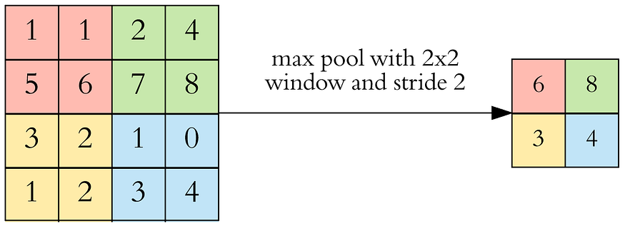
Here we have an example of maxpooling with a 2x2 window and stride 2. This pooling layer allowed us to reduce the size while also keeping the important features. Since we had a 2x2 window and a stride of 2, we essentially reduced the size of the feature map by 1/4.
Repeating the Process
Based on the architecture being implemented, a CNN will have a similar structure to going from convolution to pooling and repeating. Each architecture specifies their structure a different way.
CNN to Fully Connected Layer
As mentioned a CNN extracts features and then connects to a neural network.

Live Example
This website shows the process of a CNN really well.
Live coding
Let’s get into the live coding example. This week we will be creating a cnn to predict types of objects. We will be using the CIFAR-10 dataset to train our model. The CIFAR-10 dataset is a popular dataset that provides thousands of images on different types of objects. Let’s get started!